This post will explain steps to highlight selected row in excel. Row highlight will change dynamically based upon selection change.
This can be helpful during a meeting or discussion to keep audience focused on excel row in discussion. Find below steps to setup this functionality.
Steps: Row Highlight Configurations
- Open excel file
- Select cell range containing data
- Go to conditional formatting and select new rule. This will open new formatting rule window.

Following link to learn more about excel conditional formatting
- Select “use a fornula to determine which cells to format”. As shown below.
- Paste following formula in formula field
=ROW()=CELL("ROW")- Select format button right next to preview area
- Go to fill and select background color for the selected row

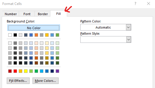
- Apply and close format cells and new formatting rule windows
- Final conditional formatting setting will look like below

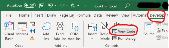
- Next go to developer tab in excel as shown below and select “View Code”
Go to link to see steps to enable excel developer tab
- Select worksheet from drop down as shown below
- This will open code block behind excel worksheet

- Add following code in code editor (as show in screenshot below)
Private Sub Worksheet_SelectionChange(ByVal Target As Range)
Target.Calculate
End Sub

- Close code editor and go back to excel sheet
- Configurations are completed. Now we can test if “Highlight selected row” configurations are working as expected.
- Select any row in the cell range that was selected for conditional formatting
- Row highlighting should dynamically change as row selection changes

Other posts from blog
- Azure Synapse Failed to List Resource Error
- Synapse SQL Authentication

2 thoughts on “Row Highlight – Excel”